Kaggle: Credit risk (Model: Support Vector Machines)
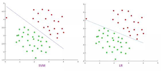
A more advanced tool for classification tasks than the logit model is the Support Vector Machine (SVM). SVMs are similar to logistic regression in that they both try to find the "best" line (i.e., optimal hyperplane) that separates two sets of points (i.e., classes).
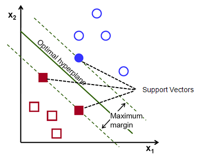
More specifically, SVMs finds a hyperplane that has the maximum margin (i.e., greatest separation) in an N-dimension space (i.e., number of features) that classifies the data points accurately. The hyperplane is of dimension N-1, thus if there are 2 (3) input features, the hyperplane is a line (two-dimensional plane). The "support vectors" relate to data points that are close to the hyper plane and can chance the orientation and position of the hyperplane. Based on these support vectors, the hyperplane can change.
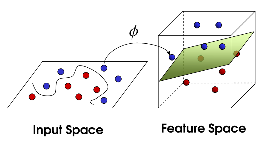
SVM uses kernel tricks to transform raw datasets in the input space into another "rich" feature space so that complex classification problems can still be solved in the same "linear" fashion based on the new alternative hyperspace. Intuitively, we can see from the above that the line separating the two classes of points is non-linear since it is 'squiggly'. The kernel trick maps raw data into another dimension that has a clear dividing linear margin between different classes of data. SVMs are unique as the mapping process from the raw data to the new dimensions are require only a user-specified kernel as opposed to a user-specified feature map.
SVM vs Logistic regression
1. Use cases
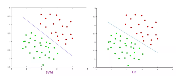
Generally, linear SVMs and logistic regression have similar performance in practice. SVMs are used when a non-linear kernel if your dataset is not linearly separable, or your model needs to be more robust to outliers. Thus one should start off with a logistic regression and advance towards a non-linear SVM with a Radial Basis Function (RBF) kernel
2. Loss functions
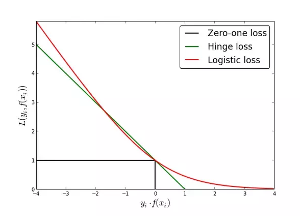
SVMs minimize a hinge loss function that maximizes the margin (i.e., largest separation) between two classes and the logit function minimizes a logistic loss function that maximizes the likelihood of posterior class probability of the points. From the figure comparing the hinge loss and logistic loss functions, we see two main differences that lead to SVM being a more robust model compared to logistic regression:
a. Accuracy
The logit function does not go to zero compared to the hinge loss function. This leads to slightly less accuracy compared to SVM.
b. Outliers
The logit function diverges more quickly than the hinge loss function. This leads to greater sensitivity to outliers compared to SVM.
3. Complexity & scalability
SVMs are more complex as can support non-linear classification. The relationship between the fit time for the SVM is more than quadratic with the number of samples. Therefore, as SVMS are less scalable compared to logistic regression, thus explaining why logit models are still commonly used as benchmark models in machine learning applications. Typically SVMs should be used on datasets of < 10,000 samples.
4. Model output
SVMs produces a binary output (i.e., 1 or 0) whereas logistic regressions produce probabilistic values of [0,1]. To obtain a binary output in logistic regression, we set a threshold such that probabilities above (below) the threshold are 1 (0).
Loading required Python modules
# importing all system modules
import os
import sys
import warnings
from pathlib import Path
warnings.filterwarnings('ignore')
if sys.platform == 'linux':
    sys.path.append('/home/randlow/github/blog2/listings/machine-learning/') # linux
elif sys.platform == 'win32':
    sys.path.append('\\Users\\randl\\github\\blog2\\listings\\machine-learning\\') # win32

# importing data science modules
import pandas as pd
import numpy as np
import sklearn
import scipy as sp
import pickleshare

# importing graphics modules
import matplotlib.pyplot as plt
import seaborn as sns

# importing personal data science modules
import rand_eda as eda
Loading pickled dataframes
To see how the below dataframes were obtained see the post on the Kaggle: Credit risk (Feature Engineering)
home = str(Path.home())
if sys.platform == 'linux':
    inputDir = "/datasets/kaggle/home-credit-default-risk" # linux
elif sys.platform == 'win32':
    inputDir = "\datasets\kaggle\home-credit-default-risk" # windows

storeDir = home+inputDir+'/pickleshare'

db = pickleshare.PickleShareDB(storeDir)
print(db.keys())

df_app_test_align = db['df_app_test_align']
df_app_train_align = db['df_app_train_align']
#df_app_train_align_expert  = db['df_app_train_align_expert']
#df_app_test_align_expert = db['df_app_test_align_expert']
#df_app_train_poly_align = db['df_app_train_poly_align']
#df_app_test_poly_align = db['df_app_test_poly_align']
Selection of feature set for model training & testing
Assign which ever datasets you want to train and test. This is because as part of feature engineering, you will often build new and different feature datasets and would like to test each one out to evaluate whether it improves model performance.
As the imputer is being fitted on the training data and used to transform both the training and test datasets, the training data needs to have the same number of features as the test dataset. This means that the TARGET column must be removed from the training dataset.
For the SVM, we use a sample of 5000 from the original dataset as fitting the SVM on all available data (i.e., 48744 entries) would be too computationally intensive.
train = df_app_train_align.copy()
test = df_app_test_align.copy()
eda.print_basic_info_df(train)
#train = train.sample(5000, random_state=50)
We see that our samples of 5000 is a fairly good representation of the original dataset given that the number of True (%) is at 7% compared to 8% in the original dataset
eda.print_basic_info_df(train)
train_labels = train.pop('TARGET')
Feature set preprocessing
from sklearn.impute import SimpleImputer
imputer = SimpleImputer(missing_values=np.nan,strategy='median')

from sklearn.preprocessing import MinMaxScaler
scaler = MinMaxScaler(feature_range= (0,1))
We fit the imputer and scaler on the training data, and perform the imputer and scaling transformations on both the training and test datasets.
imputer.fit(train)
train = imputer.transform(train)
test = imputer.transform(test)

scaler.fit(train)
train = scaler.transform(train)
test = scaler.transform(test)
Basic model
We perform a basic exercise of further splitting our training dataset into test and train datasets. Our test datasets are 20% the size of our training datasets
from sklearn.model_selection import train_test_split
X_train, X_test, y_train, y_test = train_test_split(train, train_labels, test_size=0.2, random_state=50)
from sklearn import svm
from sklearn import metrics
svm1 = svm.SVC(verbose=True)
svm1.fit(X_train,y_train)
Once we have used out trained model to predict the target label from X_test, we calculate the Accuracy and ROC AUC Score metrics. For a full range of model performance metrics see Scikit-learn: Model Evaluation
y_pred = svm1.predict(X_test)
print('Accuracy Score: {}'.format(metrics.accuracy_score(y_test,y_pred)))
print('ROC AUC Score: {}'.format(metrics.roc_auc_score(y_test,y_pred)))
We can see that our basic SVM model performs similarly to random guesses as the AUC-ROC value produced is 0.5 which means out model is performing poorly. We will first try improving our model using cross-validation and then hyper parameter tuning our model
Cross validation
We use a 10-fold cross validation to evaluate how well our model performs.
from sklearn.model_selection import cross_val_score
n_folds = 10
scores = cross_val_score(svm1, X_train, y_train, cv=n_folds, scoring='roc_auc', n_jobs=-1) #cv is cross validation
fold_names = list(range(n_folds))
fold_names.append('Average')

avg_score = scores.mean()
scores = list(scores)
scores.append(avg_score)
cv_score = pd.DataFrame({'Fold Index': fold_names, 'ROC AUC (Norm)':scores, })

cv_score
We find that on our cross validation exercise, the ROC AUC score is higher at 0.61. Cross validation has an in-sample effect, thus that may be why our model is performing better than we use a completely out of sample dataset such as X_test to obtain y_test.
Cross validation (Stratified K-fold)
Stratified K-fold differs from regular K-fold cross validation such that stratification leads to the rearrangement of the dataset to ensure that each fold is a good representative of the whole dataset For example, if we have two classes (i.e., binary classification) in our dataset where Target=1 is 30% and Target=0 is 70%, stratification will ensure that in each fold, each Target=1 and Target=0 will be accurately represented in the 30-70 context. Thus, stratification is a better scheme especially when the datasets are imbalanced (i.e., proportion of different classes are very different, 99-1) and leads to improved outcomes terms of bias and variance when compared to regular cross-validation.
from sklearn.model_selection import StratifiedKFold
strat_scores = cross_val_score(svm1,X_train,y_train,cv=StratifiedKFold(10,random_state=50,shuffle=True),scoring='roc_auc',n_jobs=-1)
avg_strat_score = strat_scores.mean()
strat_scores = list(strat_scores)
strat_scores.append(avg_strat_score)

cv_score['ROC AUC (Strat)'] = strat_scores
cv_score
We can see that the outcomes of K-fold and Stratified K-fold are similar.
Hyperparameter tuning
Most machine learning models have parameters that need to be tuned to optimize the models performance. As SVM is relatively less complicated compared to Decision Trees, Random Forest, and Gradient Boosted Trees we go through a relatively straight forward example on how to approach hyper parameter tuning.
Polynomial degrees parameter
SVMs can perform non-linear classification and this is performed using kernel=poly or kernel=rbf. Although rbf is the more popular kernel in practice, poly with a degree of 2 is often used for natural language processing. Below we explore the effect of using different polynomial degrees on the model.
degree_range=[1,2,3,4,5,6]
auc_roc_score=[]
for degree_val in degree_range:
    svc = svm.SVC(kernel='poly', degree=degree_val)
    scores = cross_val_score(svc, X_train, y_train, cv=10, scoring='roc_auc', n_jobs=-1)
    auc_roc_score.append(scores.mean())

sns.lineplot(x=degree_range,y=auc_roc_score)
From the above, we see that a polynomial degree of 2 results in the highest roc_auc score.
Gamma parameter
The gamma parameter is the inverse of the standard deviation of the RBF kernel (Gaussian function) and is used as similarity measure between two points. Thus, a small (large) value of gamma laeds to a Gaussian function with large (small) variance which intuitively means that two points can be considered similar even if they are far apart (only if they are close together).
If gamma is large, then variance is small implying the support vector does not have wide-spread influence. Technically speaking, large gamma leads to high bias and low variance models, and vice-versa.
gamma_range=[0.0001,0.001,0.01,0.1,1,10]
auc_roc_score=[]
for gamma_val in gamma_range:
    svc = svm.SVC(kernel='rbf', gamma=gamma_val)
    scores = cross_val_score(svc, X_train, y_train, cv=10, scoring='roc_auc', n_jobs=-1)
    auc_roc_score.append(scores.mean())

sns.lineplot(x=gamma_range,y=auc_roc_score)
A higher gamma leads to greater auc roc so we should use a higher value for gamma.
C parameter
C is the parameter for the soft margin cost function that controls the impact of each individual support vector. The selection of C is a trade-of between error penalty and stability. Intuitively, C is a setting that states how aggressively you want the model to avoid misclassifying each sample. Large (small) values of C lead to the optimizer seeking a small-margin (large-margin) hyperplane if this results in more accurate classification (even if this leads to greater misclassification). Thus, large (small) values of C can cause overfitting (underfitting). C needs to be selected to ensure that the trained model is generalizable to out-of-sample data points
C_range=list(range(1,30))
auc_roc_score=[]
for c in C_range:
    svc = svm.SVC(kernel='rbf', C=c)
    scores = cross_val_score(svc, X_train, y_train, cv=10, scoring='roc_auc', n_jobs=-1)
    auc_roc_score.append(scores.mean())
sns.lineplot(x=C_range,y=auc_roc_score)
We can see that using a C above 6 produces the highest roc_auc score. Thus we will select 8.
GridSearch for hyper parameter tuning
from sklearn.model_selection import GridSearchCV
tuned_parameters = {
 'C': (np.arange(5,10,1)) , 'kernel': ['linear'],
 'C': (np.arange(5,10,1)) , 'gamma': [0.01,0.1,1,2,10], 'kernel': ['rbf'],
 'degree': [2,3,4] ,'gamma': [0.01,0.1,1,2,10], 'C':(np.arange(5,10,1)) , 'kernel':['poly']
                   }

GS = GridSearchCV(svm1, tuned_parameters,cv=10,scoring='roc_auc',n_jobs=-1, verbose = True)
GS.fit(X_train,y_train)
print('The best parameters are :{}'.format(GS.best_params_))
print('The best score is: {}'.format(GS.best_score_))
y_pred= GS.predict(X_test)

print('Accuracy Score: {}'.format(metrics.accuracy_score(y_test,y_pred)))
print('ROC AUC Score: {}'.format(metrics.roc_auc_score(y_test,y_pred)))
Our SVM model performs a pretty dismal job of predicting roc_auc for out-of-sample data. We are unable to submit this data
Create the submission dataframe. We check to make sure it has the right type of data as expected by te Kaggle competition submission requirements and the right number of rows
submit = pd.DataFrame()
submit['SK_ID_CURR'] = df_app_test_align.index
submit['TARGET'] = y_pred
print(submit.head())
print(submit.shape)
We create a csv of our model output, and submit it to Kaggle.
Kaggle submission
submit.to_csv('logit-home-loan-credit-risk.csv',index=False)
!kaggle competitions submit -c home-credit-default-risk -f logit-home-loan-credit-risk.csv -m 'submitted'
The submission to Kaggle indicated that the predictive power on the test dataset was 0.6623 (66%) which is better than a 50-50 chance! Let's try a more sophisticated model.
!kaggle competitions submissions -c home-credit-default-risk
Converting iPython notebook to Python code
This allows us to run the code in Spyder.
!jupyter nbconvert ml_kaggle-home-loan-credit-risk-model-logit.ipynb --to script --output-dir='~/github/blog2/listings/machine-learning/'
Writing code into Google Drive directory for Colab
!jupyter nbconvert ml_kaggle-home-loan-credit-risk-model-logit.ipynb --to script --output-dir='/mnt/chromeos/GoogleDrive/MyDrive/Colab Notebooks'
Comments
Comments powered by Disqus