Kaggle: Credit risk (Model: Logit)
A simple yet effective tool for classification tasks is the logit model. This model is often used as a baseline/benchmark approach before using more sophisticated machine learning models to evaluate the performance improvements.
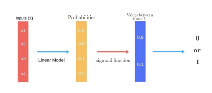
$$ \log \left( \frac{p}{1-p} \right) = \beta_0 + \beta_1 x_{1} + \beta_2 x_{2} + \beta_3 x_{3} + ... + \beta_k x_{k} $$The logistic regression takes the output of a linear function of $k$ independent variables and uses the logistic link function to output this value within the range of [0,1]. The logistic function has an "S" shape and takes a set of real values and maps it to a range of 0 to 1, but never exactly at the 0 or 1 values. Thus, the outputs of a logistic regression are probability values and we assign a value of 1 if the probability value is above a threshold value.
Logit & Sigmoid functions
The logit link function is particularly intuitive as it is $\log$ of the odds ratio. For example, given a probability $p$, the odds are calculated as $\frac{p}{1-p}$ where $p=0.8$, the odds are 4 to 1 (i.e., $0.8/0.2 = 4$).
$$ \text{Logit}(x) = \log \left(\frac{p}{1-p}\right) $$The logit function asymptotes (i.e., heads) towards $+\infty$ ($-\infty$) as p approaches 1 (0).
x = np.arange(0,1.05,0.005)
y =  np.log(x/(1-x))
df_logit = pd.DataFrame({'y_val':y },index=x)

ax = df_logit.plot(legend=False)
ax.set_title('Logit')

The inverse of the logit function is the sigmoid function. If you have a probability $p$, $\text{Sigmoid}(\text{Logit}(p))=p$. Thus, the sigmoid function maps the real values back to the range of [0,1]
$$ \text{Sigmoid}(x) = \log \left(\frac{x}{1+e^{-x}}\right) $$x = np.arange(-5,6,0.05)
y = 1/(1+np.exp(-x))
df_sigmoid = pd.DataFrame({'y_val':y },index=x)
ax = df_sigmoid.plot(legend=False)
ax.set_title('Sigmoid')

Another reason for the usefuless of the logistic (and sigmoid) function is that its gradients are easy to calculate (i.e., differentiating the function). Efficient calculation of gradients is important as optimization and machine learning techniques use gradients when estimating the optimal parameters of a model (i.e., gradient descent).
Loading in modules
# importing all system modules
import os
import sys
import warnings
from pathlib import Path
warnings.filterwarnings('ignore')
if sys.platform == 'linux':
    sys.path.append('/home/randlow/github/blog2/listings/machine-learning/') # linux
elif sys.platform == 'win32':
    sys.path.append('\\Users\\randl\\github\\blog2\\listings\\machine-learning\\') # win32

# importing data science modules
import pandas as pd
import numpy as np
import sklearn
import scipy as sp
import pickleshare

# importing graphics modules
import matplotlib.pyplot as plt
import seaborn as sns

# importing personal data science modules
import rand_eda as eda
Loading pickled dataframes
To see how the below dataframes were obtained see the post on the Kaggle: Credit risk (Feature Engineering)
home = str(Path.home())
if sys.platform == 'linux':
    inputDir = "/datasets/kaggle/home-credit-default-risk" # linux
elif sys.platform == 'win32':
    inputDir = "\datasets\kaggle\home-credit-default-risk" # windows

storeDir = home+inputDir+'/pickleshare'

db = pickleshare.PickleShareDB(storeDir)
print(db.keys())

df_app_test_align = db['df_app_test_align']
df_app_train_align = db['df_app_train_align']
#df_app_train_align_expert  = db['df_app_train_align_expert']
#df_app_test_align_expert = db['df_app_test_align_expert']
#df_app_train_poly_align = db['df_app_train_poly_align']
#df_app_test_poly_align = db['df_app_test_poly_align']
Selection of feature set for model training & testing
Assign which ever datasets you want to train and test. This is because as part of feature engineering, you will often build new and different feature datasets and would like to test each one out to evaluate whether it improves model performance.
As the imputer is being fitted on the training data and used to transform both the training and test datasets, the training data needs to have the same number of features as the test dataset. This means that the TARGET column must be removed from the training dataset.
train = df_app_train_align.copy()
test = df_app_test_align.copy()

train_labels = train['TARGET']
train = train.drop(columns=['TARGET'])
Feature set preprocessing
from sklearn.impute import SimpleImputer
imputer = SimpleImputer(missing_values=np.nan,strategy='median')

from sklearn.preprocessing import MinMaxScaler
scaler = MinMaxScaler(feature_range= (0,1))
We fit the imputer and scaler on the training data, and perform the imputer and scaling transformations on both the training and test datasets.
imputer.fit(train)
train = imputer.transform(train)
test = imputer.transform(test)

scaler.fit(train)
train = scaler.transform(train)
test = scaler.transform(test)
Model implementation (Logistic Regression)
We initialize the logistic regression with a low regularization parameter to prevent overfitting (i.e., C=0.0001) which will improve out of sample performance (i.e., performance on the test dataset)
from sklearn.linear_model import LogisticRegression

log_reg = LogisticRegression(C=0.0001)
log_reg.fit(train,train_labels)
We take the 2nd column (i.e., [:,1]) of the logistic model predictions as we are interested in predicting when the loans are in default (i.e., Target=1)
log_reg_pred = log_reg.predict_proba(test)[:,1]
Create the submission dataframe. We check to make sure it has the right type of data as expected by te Kaggle competition submission requirements and the right number of rows
submit = pd.DataFrame()
submit['SK_ID_CURR'] = df_app_test_align.index
submit['TARGET'] = log_reg_pred
print(submit.head())
print(submit.shape)
We create a csv of our model output, and submit it to Kaggle.
Kaggle submission
submit.to_csv('logit-home-loan-credit-risk.csv',index=False)
!kaggle competitions submit -c home-credit-default-risk -f logit-home-loan-credit-risk.csv -m 'submitted'
The submission to Kaggle indicated that the predictive power on the test dataset was 0.6623 (66%) which is better than a 50-50 chance! Let's try a more sophisticated model.
!kaggle competitions submissions -c home-credit-default-risk
Converting iPython notebook to Python code
This allows us to run the code in Spyder.
!jupyter nbconvert ml_kaggle-home-loan-credit-risk-model-logit.ipynb --to script --output-dir='~/github/blog2/listings/machine-learning/'
Comments
Comments powered by Disqus