Contents

In machine learning, decision trees and Classification and Regression Tree (CART) are used interchangeably. Decision trees can be used as an over-arching term to describe CARTs as Classification Trees are when the target variable takes a discrete set of values and Regression Trees when the target variable takes a continuous set of values.

Decision trees

Decision trees are simple tools that are used to visually express decision-making. For example, in Fig 1. you see a basic decision tree used to decide whether a person should be approved for a loan or not. If the applicant is less than 18 years old, the loan application is rejected immediately. If the application is between 18 and 65 years old, other conditions (i.e., family, annual income) are used to evaluate whether the application should be approved for the loan or not. In this sense, the decision tree is a set of sequential, hierarchal, decisions that lead to a final result.

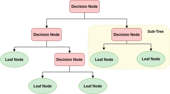
Decision trees are non-parametric as there are no underlying assumptions about the distribution of the errors or the data and the model is simply constructed based on the observed data. Commonly used terminology used in describing a decision tree are as follows:

Nodes (Split/Decision/Internal nodes): Each node represents class labels that branch off into another nodes. They are 'splitting points'.
Branches: Each branch represent 'splits' of features leading to class labels.
Leaf: These are the nodes of the tree that do not have any more additional nodes branching of them. They are basically the final nodes at the end of the tree.

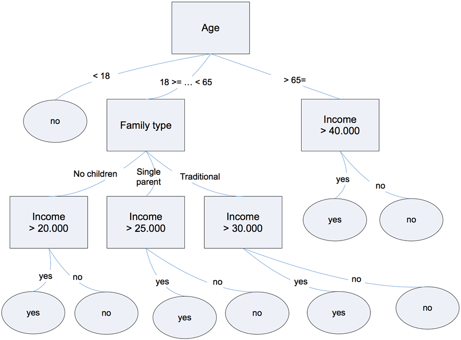
Fig 2. Decision Tree for loan approvals

Building a decision tree

Constructing a decision tree is a 2-step process as follows:

Induction

Induction is where the tree is actually built and where we set all the hierarchal decision boundaries based on our data.

Determine the "best" feature in the dataset to split the data on.
Define a node on the tree by splitting the dataset into subsets that contain the range of values for the "best" feature.
Recursively create new tree nodes based on the data created from Step 2. Splitting of data (i.e., creation of new nodes) into subsets continues to the point where the optimal maximum accuracy has been achieved, while minimizing the number of "splits"/nodes.

Cost function

Selecting the best feature to split on and where to split it is chosen using a greedy algorithm to minimize a cost function. The cost function for a regression tree can be squared error:

\begin{equation*} \epsilon_{reg} = \sum^{N}_{i=1} (y-\hat{y})^2 \end{equation*}

where \(y\) are the predicted values from the model, and \(\hat{y}\) are the observed values from the dataset. By summing over all \(N\) observations of the differences between the model's predicted values and observed values, the total error of our model is calculated. The model is optimized to minimize the error value.

The cost function for a classification tree can be the

Gini Index

\begin{equation*} \epsilon_{gini} = 1- \sum^{C}_{i=1} p_{i}^{2} \end{equation*}

The Gini index score informs how good a split is based on how mixed the number of classes are in the the groups created by the split. \(p_i\) is the proportion of instances of class \(i\) for a particular group and \(C\) is the total number of classes. As an example, for a set of items with 2 classes (i.e., 1 and 0), perfect class purity (\(\epsilon_{gini}=0\)) occurs when a group contains all inputs from the same class such that \(p_i\) is either 1 or 0 (i.e., binary classifier). If class purity is low (\(\epsilon_{gini}=0.5\)) then there is a 50-50 split of classes in a group and \(p_i\) is 0.5. The split point is selected based on the minimum gini index.

Information Gain

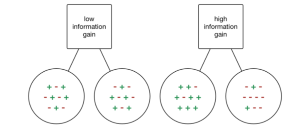
\begin{equation*} \epsilon_{gini} = -\sum^{C}_{i=1} p_{i} \log p_{i} \end{equation*}

Fig 3. Information gain

The information gain is intuitively shown in Fig 2. We can see that the node with low information gain has a more or less equivalent number of + and - in both branches. The node with high information gain has a more larger number of + on the left branch and more - on the right branch. Thus, the node with the high information gain is more useful as we have gained more information since we know that feature clearly splits out dataset more distinctly into the two groups of + and -. Nodes with low information gain are less useful as they do not clearly de-lineate the data into the two groups. Information gain is based on the concept of entropy (i.e., impurity of an input set) and a simplified formula is as below:

\begin{equation*} \text{Information Gain} = \text{Entropy(parent)} - \text{Weighted Sum of Entropy (Children)} \end{equation*}

Stopping method

Minimum number of observations per group: Set a minimum number of observations assigned to each leaf node. Thus, when a node is being evaluated as it will only split if the number of observations is more than the minimum number, and turn into a leaf node otherwise. A smaller minimum set for the splitting threshold will lead into finer splits, more information, but also potential overfitting on your dataset.
Maximum tree depth: Set the maximum length of the longest path from the root of the tree to a leaf to a specified number.

Pruning

Pruning is the process of removing any unnecessary structures (i.e., leaves and nodes) from the decision tree. This is to reduce model complexity and prevent model overfitting. It also helps with improving the interpretability of the model. A simple pruning method is to remove each leaf node in the tree and evaluate the effect of doing so on a hold-out test dataset. If there is a drop in the overall cost function on the entire test dataset, then the leaf node is removed.

Comments