Contents

A crucial concept in machine learning is understanding the cost function and gradient descent. Intuitively, in machine learning we are trying to train a model to match a set of outcomes in a training dataset. The difference between the outputs produced by the model and the actual data is the cost function that we are trying to minimize. The method to minimize the cost function is gradient descent. Another important concept is gradient boost as it underpins the some of the most effective machine learning classifiers such as Gradient Boosted Trees.

Cost function

A cost function is a value that we want to minimize. In machine learning, we want to minimize the sum of squared errors (MSE) between the outputs produced by our model and the actual data itself. Thus, machine learning is about finding and fitting a model that produces output values (\(Y_{i}\)) that are as close as possible to the actual data (\(\hat{Y_{i}}\)) as shown below:

\begin{equation*} MSE = \frac{1}{N} \sum^N_{i=1} (Y_{i}-\hat{Y}_{i})^2 \end{equation*}

With some mathematical adjustments we obtain the following where the data points output by the model is given by \(h_\theta(x^{(i)}\) and the actual data points are \(y^{(i)}\). Below is the mathematical equation often shown in machine learning courses.

\begin{equation*} MSE = \frac{1}{2m} \sum^m_{i=1} (h_\theta(x^{(i)})-y^{(i)})^2 \end{equation*}

Gradient descent (GD)

Gradient descent

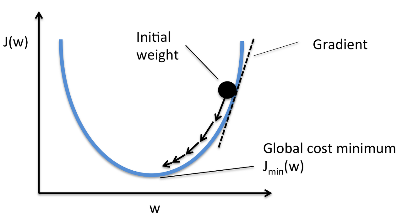
\begin{equation*} \min_{\Theta} J(\Theta) = \frac{1}{2m} \sum^m_{i=1} (h_\theta(x^{(i)})-y^{(i)})^2 \end{equation*}

To minimize the cost function, we use gradient descent. Gradient Descent is a general function for minimizing a function, in this case the Mean Squared Error (MSE) cost function. Gradient Descent allows us to find the global minima for our cost function by changing the parameters (i.e., \(\Theta\) parameters) in the model slowly until we have arrived at the minimum point. The gradient descent formula is shown as follows.

\begin{equation*} \Theta_{j} := \Theta_{j} -\alpha \frac{\partial J(\Theta_0,\Theta_1)}{\partial \Theta_{i}} (\text{for} j=0, j=1) \end{equation*}

\(\alpha\) is the learning rate. It indicates how quickly we move to the minimum and if it is too large we can overshoot. Having a very small learning rate mean that the model might converge too slowly.

Intutively, if the cost is a function of \(K\) variables, then the gradient is the length-\(K\) vector that defines the direction that the cost is increasing most rapidly (i.e., \(\frac{\partial J(\Theta_0,\Theta_1)}{\partial \Theta_{i}}\)). With gradient descent, you follow the negative of the gradient to the point where the cost is a minimum. Thus, the set of parameters (\(\Theta\)) is updated in an iterative manner to minimize the cost function.

With gradient descent, it is necessary to run through all of the samples in the training data to obtain a single update for a parameter in a particular iteration. Samples are selected in a single group or in the order they appear in the training data. Thus, if you have a large dataset, the process of gradient descent can be much slower.

Stochastic Gradient Descent (SGD)

Most machine learning models are using stochastic gradient descent because it is a faster implementation. SGD uses only one or a subset of the training sample from the training dataset to perform an update for the parameters in a particular iteration. It is called stochastic as samples are selected randomly,

SGD converges faster than GD, but the cost function may not be as well minimized as GD. However, the approximation obtained for model parameters is close enough to the optimal values given it is a much quicker implementation. SGD is the de facto training algorithm for artificial neural networks.

Gradient Boost

Previously, when we optimize for a cost function, the function remains static (\(F\)) and the parameters (\(P\)) are updated to minimize the cost function as shown below:

\begin{equation*} F(x|P) = \min_{P} \text{Loss}(y,F(x|P)) \end{equation*}

With gradient boosting, both the function and the parameters are being optimized. This is a much more complex problem as previously the number of parameters being optimized was fixed since the function does not change. However, now my number of parameters being optimized can change as the function itself can change too.

\begin{equation*} F(x|P) = \min_{F,P} \text{Loss}(y,F(x|P)) \end{equation*}

In previous implementations, SGD or GD is ued to train a single complex model. Gradient boosting finds the best function \(F\) by combining many simple functions together (i.e., an ensemble of simple models).

Cost function

Gradient descent (GD)

Stochastic Gradient Descent (SGD)

Gradient Boost

Comments