This is an overview of the diagnostic and performance tests that need to be performed to ensure the validity of a time-series ARIMAX regression model.

\begin{equation*} R_{t} = \mu + \sum^{p}_{i=1} \alpha_{i} R_{t-i} + \sum^{q}_{j=1} \beta_{j} \epsilon_{t-j} + \sum^{r}_{k=1} \gamma_{k} X_{t,k} + \epsilon_{t} \text{, where } \epsilon \backsim N(0,\sigma) \end{equation*}

In the above equation, $R_{t}$ is the differenced original series. For example, if we have stock prices ($P_{t}$), we perform a differencing operation of 1 (i.e., $R_{t} = P_{t} - P_{t-1}$).

A time series is integrated of order $d$ if $(1-L)^{d} X_{t}$ is a stationary process where $L$ is the lag operator and $1-L$ is the first difference (i.e., $(1-L)X_{t}=X_{t}-X_{t-1}$). A time series of order $d=2$ is as follows:

\begin{equation*} \triangle^{2} R_{t} = \triangle Y_{t} - \triangle Y_{t-1} \end{equation*}

The values of $p$ and $q$ are the orders of the autoregressive (AR) and moving average (MA) terms. The value of $r$ denotes the number of independent variable (X) terms included in the model.

5 minute read…

Why should we do our own automated trading?

Rand Low

2019-Mar-01

Comments

Contents

Many people often ask me several questions about why we should even bother doing our own automated trading.

Why not let the professionals do it?

There's really nothing wrong with letting your money sit in a managed fund. However, let me pose the same questions and frame them differently:

Why do some people file their own taxes annually to the ATO? Why not give it to the accountant?
Why do gym-goers create their own exercise plans and go to the gym? Why not get a trainer to create your exercise plan and guide you through the process?
Why do some investors choose to buy/sell & manage their own rental properties? Why not let a real estate agent do it?
(Put your own example here)

I suppose you can see where I am going with this.

3 minute read…

Hybrid machine learning solution with Google Colab

Rand Low

2019-Feb-12 (updated 2019-Feb-15)

Comments

jupyterlab colab gcp

Google Colab is an excellent free resource provided by Google to use GPUs or TPUs for training your own machine learning models or performing quantitative research. Personally, I have a hybrid solution of performing EDA on the dataset, feature engineering, before transitioning to Google Colab for model selection and hyper parameter tuning.

Google Colab really is a game changer as basically anyone with a cheap laptop and an internet connection can have access to some of the most powerful processors for some heavy duty number-crunching, whether that's optimising a trading model or training a machine learning model to identify images, or performing natural language processing on a ton of websites or documents. Of course, what they are hoping for is that quantitative finance professionals, data scientists, and academics will eventually opt for using the Google Cloud Platform if they need even more processing power. But ultimately, all of these free resources does democratize programming and machine learning etc., so we're all better off for it.

With Colab, you can request GPUs (NVIDIA Tesla K80 GPU) and TPUs and use them for a maximum of 12 hours.

Hybrid cloud workflow for Python¶

Using the Files app of ChromeOS, create a folder called Colab Notebooks. This is where we can store any of our iPython Notebooks and Python scripts (e.g., ipynb, py).
Create a subfolder within Colab Notebooks called datasets. This is where our datasets are stored.
Create a subfolder within Colab Notebooks called modules. This is where our personal Python modules are stored.

In [ ]:

.
└── Colab Notebooks
    ├── datasets
    └── modules

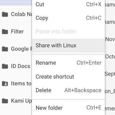
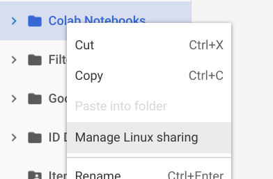
In the Files app, right-click the Colab Notebooks folder and select Share with Linux. You can now access this folder in the /mnt/chromeos/ directory in Crostini.

linux share

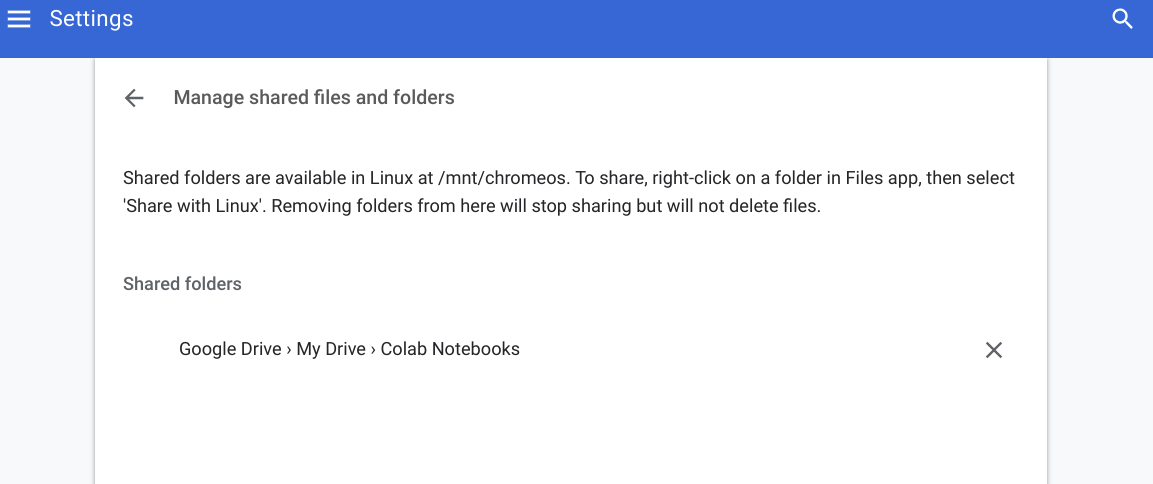
To stop sharing any folders/files from being shared with Linux, enter the Settings in ChromeOS and select the Manage shared files and folders. You can remove any folders/files that are being shared between both systems from here.

linux_manage

Code: Working locally and in Colab¶

GitHub:
- Code that is stored in a GitHub public repository can be directly pulled.
Google Drive:
- Copy your iPython notebook or Python script into the Colab Notebooks directly.
- Run the nbconvert command to output Python script into the shared folder as shown below

In [ ]:

!jupyter nbconvert ml_kaggle-home-loan-credit-risk-model-logit.ipynb --to script --output-dir='/mnt/chromeos/GoogleDrive/MyDrive/Colab Notebooks`

Datasets: Working locally and in Colab¶

As the folder \Colab Notebooks\datasets is in Google Drive, it can be accessed locally on your Chromebook and also from CoLab

Mount Google Drive to your Colab runtime instance¶

In [1]:

from google.colab import drive
drive.mount('/content/gdrive')

Go to this URL in a browser: https://accounts.google.com/o/oauth2/auth?client_id=947318989803-6bn6qk8qdgf4n4g3pfee6491hc0brc4i.apps.googleusercontent.com&redirect_uri=urn%3Aietf%3Awg%3Aoauth%3A2.0%3Aoob&scope=email%20https%3A%2F%2Fwww.googleapis.com%2Fauth%2Fdocs.test%20https%3A%2F%2Fwww.googleapis.com%2Fauth%2Fdrive%20https%3A%2F%2Fwww.googleapis.com%2Fauth%2Fdrive.photos.readonly%20https%3A%2F%2Fwww.googleapis.com%2Fauth%2Fpeopleapi.readonly&response_type=code

Enter your authorization code:
··········
Mounted at /content/gdrive

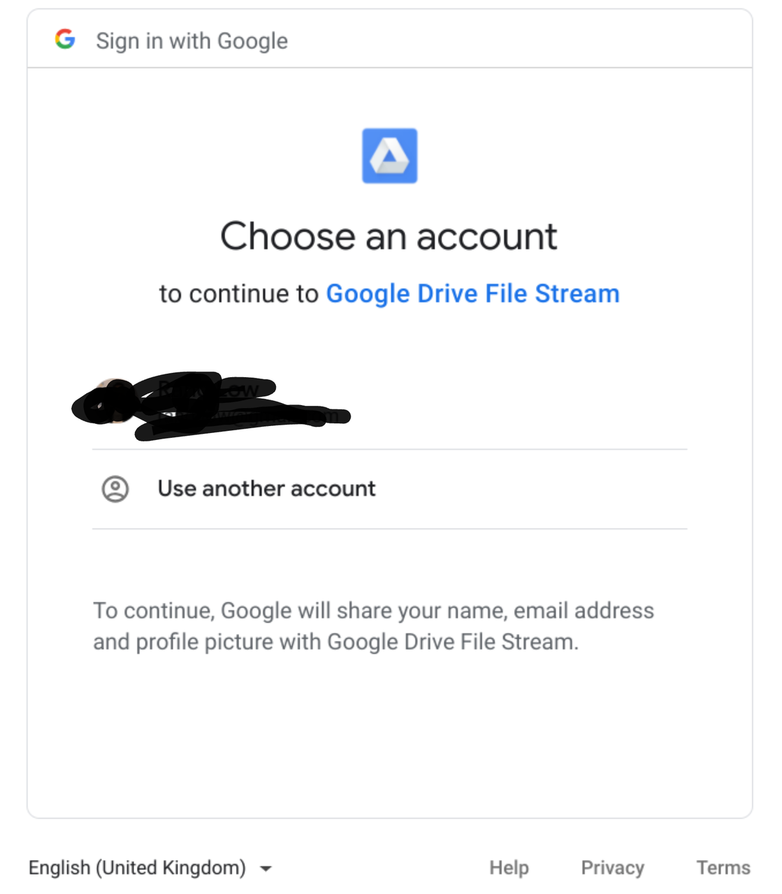
Click the link provided to you, and a new tab will open requesting that you select a Google Account to access Google Drives with.

account

Upon selecting an account, you need to authorize Google Cloud to interface with Google Drives.

authorization

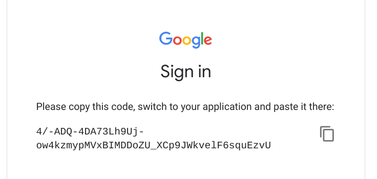
Once you've authorized the action, you will be brought to another page that has a token. This token needs to be copied and pasted in our Colab. At that point, you will be able to access all files in your Google Drive from your runtime instance.

code

Loading your datasets into Google Colab¶

As the Google Drive is successfully mounted, we go into the directory where our files are stored. In my specific instance, my datasets are stored in Colab Notebooks/datasets/kaggle/, and I am using pickle to extract datasets that I have stored earlier. Obviously you can use pd.read_csv if you have csv files in your Google Drive since it is now mounted on your runtime instance.

In [3]:

import pickleshare

inputDir = "/content/gdrive/My Drive/Colab Notebooks/datasets/kaggle/home-credit-default-risk"
storeDir = inputDir+'/pickleshare'

db = pickleshare.PickleShareDB(storeDir)
print(db.keys())

['df_app_test_align', 'df_app_train_align', 'df_app_train_corr_target', 'df_app_train_align_expert', 'df_app_test_align_expert', 'df_app_train_poly_align', 'df_app_test_poly_align']

Loading your Python modules into your Colab runtime instance¶

The easiest way is to use the sys module and append the module directory or the directory where all your notebooks and scripts are stored in your Google Drive

In [ ]:

import sys
sys.path.append('/content/gdrive/My Drive/Colab Notebooks/module') # modules
sys.path.append('/content/gdrive/My Drive/Colab Notebooks') # colab

Now you can load in your own modules easily!

In [ ]:

import rand_eda as eda

Conclusion¶

There you go! Now you know how to have a hybrid workflow to combine working on Python locally on your machine and also on Colab! You've learnt how to perform the following:

Share folders/files between Google Drive in ChromeOS and Crostini (Linux Container)
Mount Google Drives into your Colab run instance
Append a directory that stores your own Python modules into the Python path

How many neurons and layers for a multilayer perceptron (MLP)?

Rand Low

2019-Feb-09

Comments

This is a question that is often posed by many machine-learning beginners. The answer is that there are only rules of thumb and it is a trial and error process to optimize your neural network for your specific application.

2 minute read…

Bayes' theorem

Rand Low

2019-Jan-30 (updated 2019-Feb-02)

Comments

Bayes' theorem is a mathematical equation used in probability and statistics ot calculate conditional probability. Intuitively, it is used to calculate the probability of an event, based upon it's association with another event.

\begin{equation*} P(A|B)= P(B|A)\frac{P(A)}{P(B)} \end{equation*}

$P(A|B)$ is the probability of A occuring, given that B is true. $P(A)$ and $P(B)$ are the probabilities of A and B occuring independently of each other.

Example

Let's say we want to have the probability of having the flu if a child has a running nose.

$A$ is the event that a child has a flu, and the probability of this event is 20%. $P(A)=0.2$.
$B$ is the event that a child has a running nose, and the probability of this event is 50%. $P(B)=0.5$.
Research indicates that 20% of children have a running nose (B) due to the flu (A). $P(B|A)=0.2$

When we insert these values into the theorem:

\begin{equation*} P(\text{Flu}|\text{RunnyNose}) = P(\text{RunnyNose}|\text{Flu}) \frac{P(\text{Flu})}{P(\text{RunnyNose})} \end{equation*}

\begin{equation*} P(\text{Flu}|\text{RunnyNose}) = 0.2 \times \frac{0.2}{0.5} \end{equation*}

\begin{equation*} P(\text{Flu}|\text{RunnyNose}) = 0.08 \end{equation*}

Therefore, there is an 8% probability that a child who has the flu when they have the running nose. This indicates that it is unlikely that a random patient with running nose has the flu since the probability is only 0.08.

Impact of sensitivity and specificity

Bayes' theorem demonstrates the effect of false positives and false negatives.

Sensitivity: This is the true positive rate (TPR). It is the measure of the proportion of correctly identified positives. A sensitive test rarely misses a "positive".
Specificity: This is the true negative rate (TNR). It is the measure of the proportion of correctly identified negatives. A specific test rarely misses a "negative".

A prefect test is 100% sensitive and specific; however, most tests have a minimum error called the Bayes Error Rate. Below is the Bayes' Theorem re-written in a form that is usually used to solve the accuracy of medical tests.

\begin{equation*} P(A|X)=\frac{P(X|A) P(A)}{P(X|A)P(A)+P(X|\sim A)P(\sim A)} \end{equation*}

In real-world applications, a trade-off is based between sensitivity (TPR) and specificity (TNR) depending on whether it is more important to not miss a positive result, or whether its better to not label a negative result as positive.

Cluster analysis

Rand Low

2019-Jan-30 (updated 2019-Feb-02)

Comments

Cluster analysis is a technique used to group similar observations into a number of clusters based on the observed values of several variables for each individual observation. The group membership of the sample of observations is unknown prior to the algorithm being used, therefore clustering is a method of unsupervised learning.

Clustering algorithms identify clusters based on a distance metric that measures how similar different observations in the dataset are to each other.

Two major distance metrics are:

Euclidean distance: This is the distance between the two points which is the hypotenuse of a triangle ABC that connects the two points $X$ and $Y$. Euclidean distance is sensitive to the scales of the variables being used, and is blind to correlated variables.

\begin{equation*} D(i,j) = \sqrt{A^2+B^2} = \sqrt{(X_{2}-X_{1})^2+(Y_{2}-Y_{1})^2} \end{equation*}

Mahalanobis distance: This takes into account co-variances that lead to elliptic decision boundaries, as opposed to circular boundaries in the Euclidean case. As such, problems of scale and correlation in Euclidean distance are no longer an issue.

\begin{equation*} D = \sqrt{ (x-\mu)^\intercal \times C^{-1} \times (x-\mu)} \end{equation*}

where $D$ is the Mahalanobis distance, $x-\mu$ is the distance of the vector of points from the mean, $C$ is the covariance matrix of independent variables, $x$ is the vector of observations, and $\mu$ are the mean values of the independent variables.

Several clustering algorithms (and more!) are available via scikit-learn clustering and we explain several below.

4 minute read…

kNN vs k-Means

Rand Low

2019-Jan-30 (updated 2019-Feb-02)

Comments

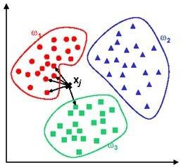
k-NN: Classification algorithm, and is a subset of supervised learning. k-NN is for number of nearest neighbors. For example, you already have a set of identified clusters groups and you have a new point added to your data set. Thus, you want to know which cluster your new point belongs to. Therefore, you see how many neighbors your new point has in which cluster.

For example, if you have a 5-NN as in 5 nearest neighbors, it detects that out of the 5 closest neighbours, 4 are in $\omega_1$ and 1 are in $\omega_3$, therefore your new point belongs to $\omega_1$.

k-Means: Clustering algorithm, and is a subset of unsupervised learning. $k$ refers to the defined number of clusters for the algorithm. K-means is a family of moving centroid algorithms, such that at every iteration the center of the cluster moves slightly to minimize the objective function. This continues until (i) the means stop changing (ii) the maximum nunber of iterations has been reached.

Kaggle: Credit risk (Model: Gradient Boosting Machine - LightGBM)

Rand Low

2019-Jan-22 (updated 2019-Jan-25)

Comments

A more advanced model for solving a classification problem is the Gradient Boosting Machine. There are several popular implementations of GBM namely:

XGBoost - Released by Tianqi Chen (March, 2014)
Light GBM - Releast by Microsoft (Jan, 2017)
CatBoost - Released by Yandex (April, 2017)

Each of the packages differ how they choose to split the decision trees within the ensemble and how categorical variables a treated. My review through the internet is that the accuracy of these different Gradient Boosting packages are somewhat similar, and they differ mainly in terms of implementation speed. A crucial component of these different packages is how they treat and process categorical variables.

We will explore Light Gradient Boosting Machine (LGBM) in our below implementation.

Loading in required modules¶

In [11]:

# importing all system modules
import os
import sys
import warnings
import ipdb
from IPython.core.debugger import set_trace
from pathlib import Path
warnings.filterwarnings('ignore')
if sys.platform == 'linux':
    sys.path.append('/home/randlow/github/blog2/listings/machine-learning/') # linux
elif sys.platform == 'win32':
    sys.path.append('\\Users\\randl\\github\\blog2\\listings\\machine-learning\\') # win32

# importing data science modules
import pandas as pd
import numpy as np
import sklearn
import scipy as sp
import pickleshare

# importing graphics modules
import matplotlib.pyplot as plt
import seaborn as sns


# importing personal data science modules
import rand_eda as eda

Loading pickled dataframes¶

To see how the below dataframes were obtained see the post on the Kaggle: Credit risk (Feature Engineering)

In [15]:

if sys.platform == 'linux':
    inputDir = "/mnt/chromeos/GoogleDrive/MyDrive/Colab Notebooks/datasets/kaggle/home-credit-default-risk" # linux
    storeDir = inputDir+'/pickleshare'
elif sys.platform == 'win32':
    home = str(Path.home())
    inputDir = "\datasets\kaggle\home-credit-default-risk" # windows
    storeDir = home+inputDir+'\pickleshare'

print(storeDir)

/mnt/chromeos/GoogleDrive/MyDrive/Colab Notebooks/datasets/kaggle/home-credit-default-risk/pickleshare

In [16]:

db = pickleshare.PickleShareDB(storeDir)
print(db.keys())

['df_app_test_align', 'df_app_train_align', 'df_app_train_corr_target', 'df_app_train_align_expert', 'df_app_test_align_expert', 'df_app_train_poly_align', 'df_app_test_poly_align']

In [17]:

df_app_test_align = db['df_app_test_align'] 
df_app_train_align = db['df_app_train_align'] 
#df_app_train_align_expert  = db['df_app_train_align_expert'] 
#df_app_test_align_expert = db['df_app_test_align_expert'] 
#df_app_train_poly_align = db['df_app_train_poly_align']
#df_app_test_poly_align = db['df_app_test_poly_align']

Assign which ever datasets you want to train and test. This is because as part of feature engineering, you will often build new and different feature datasets and would like to test each one out to evaluate whether it improves model performance.

As the imputer is being fitted on the training data and used to transform both the training and test datasets, the training data needs to have the same number of features as the test dataset. This means that the TARGET column must be removed from the training dataset, and stored in train_labels for use later.

In [18]:

train = df_app_train_align.copy()
test = df_app_test_align.copy()

labels = train.pop('TARGET').values # store training labels
feat_names = list(train.columns) # store feature names

In [19]:

train_ids = train.index.values
test_ids = test.index.values

Feature set preprocessing¶

In [20]:

from sklearn.impute import SimpleImputer
imputer = SimpleImputer(missing_values=np.nan,strategy='median')

from sklearn.preprocessing import MinMaxScaler
scaler = MinMaxScaler(feature_range= (0,1))

We fit the imputer and scaler on the training data, and perform the imputer and scaling transformations on both the training and test datasets.

Scikit-learn models only accepts arrays. So the imputer and scalers can accept DataFrames as inputs and they output the train and test variables as arrays for use into Scikit-Learn's machine learning models.

In [21]:

imputer.fit(train)
train = imputer.transform(train)
test = imputer.transform(test)

scaler.fit(train)
train = scaler.transform(train)
test = scaler.transform(test)

In [22]:

train.shape

Out[22]:

(307511, 236)

Model implementation (Gradient Boosting Machine)¶

With the Gradient Boosting machine, we are going to perform an additional step of using K-fold cross validation (i.e., Kfold). In the other models (i.e., Logit, Random Forest) we only fitted our model on the training dataset and then evaluated the model's performance based on the test dataset.

Using Kfold, we are going to split up our test data set into multiple folds (i.e., $K$). We will be fitting our model on $K-1$ folds and testing it on the $K^{th}$ fold (i.e., out-of-fold) and repeating the fitting process until all $K$ folds are explored. This method allows us to train our model more accurately without overfitting.

Thus, we copy our train (test_feat) dataframe to feat (test_feat) as these are more accurate descriptors since they are now feature and test feature datasets. The training dataset is split into further training and validation datasets based on the kfold.

In [23]:

feat = train.copy()
test_feat = test.copy()

In [ ]:

from sklearn.model_selection import KFold
from sklearn.metrics import roc_auc_score
import lightgbm as lgb
import gc

Initialization of empty variables for kfold operation

In [ ]:

feat_imp_vals = np.zeros(len(feat_names)) # feature importance
test_pred = np.zeros(test_feat.shape[0]) # test predictions
oof = np.zeros(feat.shape[0]) # out of fold predictions
valid_scores = [] # validation scores
train_scores = [] # training scores
n_folds = 5

In [ ]:

k_fold = KFold(n_splits = n_folds, shuffle=True,random_state=100)

With the KFold we are taking our training dataset, and splitting it into further training and validation datasets. The k_fold

n_estimators: Number of boosted trees to fit (i.e., 1000 trees).
reg_alpha: L1 regularization on weights (i.e., LASSO).
reg_lambda: L2 regularization on weights (i.e, Ridge.
subsample: Subsample ratio of training instance. Setting it to 0.5 lgb will randomly sample half of the training data prior to growing trees. and this will prevent overfitting. Subsampling will occur once in every boosting iteration. This prevents overfitting of the tree.
learning_rate: Boosting learning rate.
n_job : Number of processes to use for calculation. -1 means all processes will be used.
random_state : Allows model fit to be replicated.
class_weight :

In [ ]:

for train_indices, valid_indices in k_fold.split(feat):
    
    train_feat, train_labels = feat[train_indices], labels[train_indices] # training data for the fold
    valid_feat, valid_labels = feat[valid_indices], labels[valid_indices] # validation data for the fold
    
    model = lgb.LGBMClassifier(n_estimators=1000, objective='binary',
                              class_weight='balanced',learning_rate=0.05,
                              reg_alpha = 0.1, reg_lambda=0.1,
                              subsample = 0.8, n_jobs = -1, random_state=50)


    model.fit(train_feat, train_labels, eval_metric = 'auc',
              eval_set = [(valid_feat, valid_labels), (train_feat, train_labels)],
              eval_names = ['valid','train'], early_stopping_rounds = 100, verbose = 200)
             # categorical_feature = cat_indices,
    
    # record best iteration of each fold
    best_iter = model.best_iteration_ 
    # record the most important features of each fold
    feat_imp_vals += model.feature_importances_/k_fold.n_splits 
    # record the out-of-fold predictions
    oof[valid_indices] = model.predict_proba(valid_feat, num_iteration = best_iter)[:,1]/k_fold.n_splits
    
    # record the predictions on the test_feat dataset
    test_pred += model.predict_proba(test_feat, num_iteration =  best_iter)[:,1]/k_fold.n_splits 
    
    valid_score = model.best_score_['valid']['auc']
    train_score = model.best_score_['train']['auc']
    
    valid_scores.append(valid_score)
    train_scores.append(train_score)
    
    gc.enable()
    del model, train_feat, valid_feat
    gc.collect()

Training until validation scores don't improve for 100 rounds.

Creating summary of validation and training AUC scores¶

In [15]:

valid_auc = roc_auc_score(labels,oof) # calculate the auc based on the test dataset labels and the out-of-fold predictions
valid_scores.append(valid_auc) # calculate the overall validation auc score
train_scores.append(np.mean(train_scores)) # calculate the overall average training auc score

fold_names = list(range(n_folds))
fold_names.append('overall')

metrics = pd.DataFrame({'fold': fold_names,
                      'train': train_scores,
                      'valid': valid_scores})

Showing important features of the dataset¶

In [26]:

feat_imp = pd.DataFrame({'Feature': feat_names,'Importance':feat_imp_vals}) # creating feature importance dataframe
eda.plot_feat_importance(feat_imp)

Creating submission dataframe¶

In [15]:

submission = pd.DataFrame({'SK_ID_CURR': test_ids, 'TARGET': test_pred}) # creating Kaggle submission dataframe

Kaggle submission¶

We create the submission dataframe as per the Kaggle home-credit-default-risk competition guidelines

In [18]:

submit = submission
print(submit.head())
print(submit.shape)

   SK_ID_CURR    TARGET
0      100001  0.278467
1      100005  0.499217
2      100013  0.179013
3      100028  0.253097
4      100038  0.672102
(48744, 2)

Submit the csv file to Kaggle for scoring

In [22]:

submit.to_csv('lightgbm-home-loan-credit-risk.csv',index=False)
!kaggle competitions submit -c home-credit-default-risk -f lightgbm-home-loan-credit-risk.csv -m 'submitted'

100%|██████████████████████████████████████| 1.22M/1.22M [00:01<00:00, 1.07MB/s]
Successfully submitted to Home Credit Default Risk

We review our Light GBM from Kaggle and find that there is a slight improvement to 0.74 compared to 0.662 (logit) or 0.688 (random-forest). We can see that substantial improvements are obtained using LightGBM with the same dataset as logit or random-forest leading us to understand why Gradient Boosted Machines are the machine learning model of choice for many data scientists.

In [31]:

!kaggle competitions submissions -c home-credit-default-risk

fileName                                 date                 description  status    publicScore  privateScore  
---------------------------------------  -------------------  -----------  --------  -----------  ------------  
lightgbm-home-loan-credit-risk.csv       2019-02-19 04:16:44  submitted    complete  0.74158      0.74351       
random-forest-home-loan-credit-risk.csv  2019-02-19 04:15:01  submitted    complete  0.74158      0.74351       
random-forest-home-loan-credit-risk.csv  2019-02-11 17:31:03  submitted    complete  0.68694      0.68886       
random-forest-home-loan-credit-risk.csv  2019-02-11 05:24:55  submitted    complete  0.68694      0.68886       
random-forest-home-loan-credit-risk.csv  2019-02-11 05:10:40  submitted    complete  0.68694      0.68886       
logit-home-loan-credit-risk.csv          2019-02-11 04:52:51  submitted    complete  0.66223      0.67583       
random-forest-home-loan-credit-risk.csv  2019-02-11 04:44:50  submitted    complete  0.68694      0.68886       
logit-home-loan-credit-risk.csv          2019-02-08 04:08:33  submitted    complete  0.66223      0.67583

Converting iPython notebook to Python code¶

This allows us to run the code in Spyder.

In [32]:

!jupyter nbconvert ml_kaggle-home-loan-credit-risk-model-lightgbm.ipynb --output-dir='~/github/blog2/listings/machine-learning/' --to python

[NbConvertApp] Converting notebook ml_kaggle-home-loan-credit-risk-model-lightgbm.ipynb to python
[NbConvertApp] Writing 10474 bytes to /home/randlow/github/blog2/listings/machine-learning/ml_kaggle-home-loan-credit-risk-model-lightgbm.py

In [ ]:

Hybrid cloud workflow for Python¶

Sharing files between ChromeOS and Crostini (Linux container)¶

Code: Working locally and in Colab¶

Datasets: Working locally and in Colab¶

Mount Google Drive to your Colab runtime instance¶

Loading your datasets into Google Colab¶

Loading your Python modules into your Colab runtime instance¶

Conclusion¶

Example

Impact of sensitivity and specificity

Loading in required modules¶

Loading pickled dataframes¶

Feature set preprocessing¶

Model implementation (Gradient Boosting Machine)¶

Creating summary of validation and training AUC scores¶

Showing important features of the dataset¶

Creating submission dataframe¶

Kaggle submission¶

Converting iPython notebook to Python code¶