Kaggle: Credit risk (Exploratory Data Analysis)

An important topic in regulatory capital modelling in banking is the concept of credit risk. Credit risk is the loss to a bank's portfolio of loans when their customers start to default on their loans (i.e., not pay their loan repayments, or missing their repayments). These loans can be home loans, credit cards, car loans, personal loans, corporate loans, etc. (i.e., mortgages, revolving lines of credit, retail loans, whole sale loans). Credit risk is also related to securitized products and a a related post is on capital modelling as applied to securitized financial products.
22 minute read…

Machine learning model peformance metrics

Using the right metrics for our machine learning model and the dataset that is being explored is important. It is particularly important to understand the elements of the confusion matrix as several metrics are calculated based on it. Other popular metrics are the ROC-AUC and log-loss metric


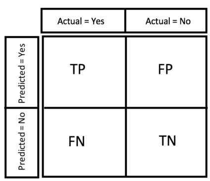
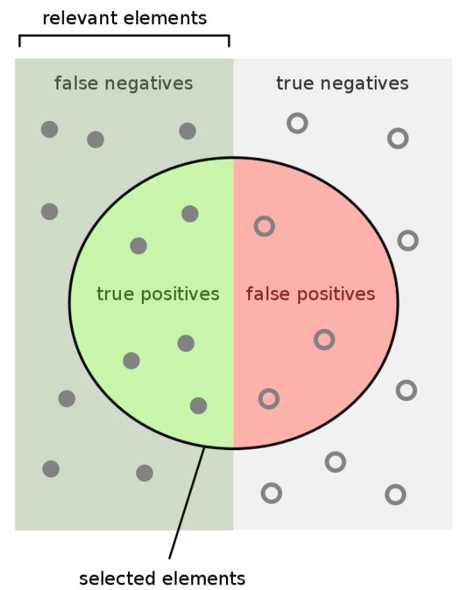
Confusion Matrix

/images/ml/ml_confusion_matrix.png
True Positive (TP)

Number of cases that are predicted as True and are actually True.

True Negative (TN)

Number of cases that are predicted as False and are actually False.

False Positive (FP)

Number of cases are are predicted as True and are actually False.

False Negative (FN)

Number of cases that are predicted as False and are actually True.

Confusion Matrix Metrics

/images/ml/ml_metric_diag.png
Accuracy

Percentage of items classified accurately. \(\frac{TP+TN}{TP+TN+FP+FN}\)

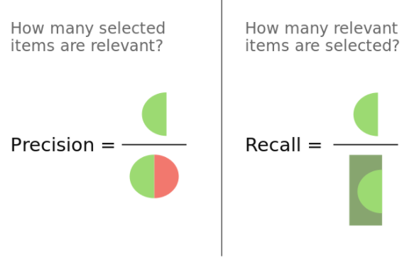
/images/ml/ml_precision_recall.png
Precision (P)

Fraction of predicted positive events that are actually positive (i.e., how correct is the model?). \(\frac{TP}{TP+FP}\)

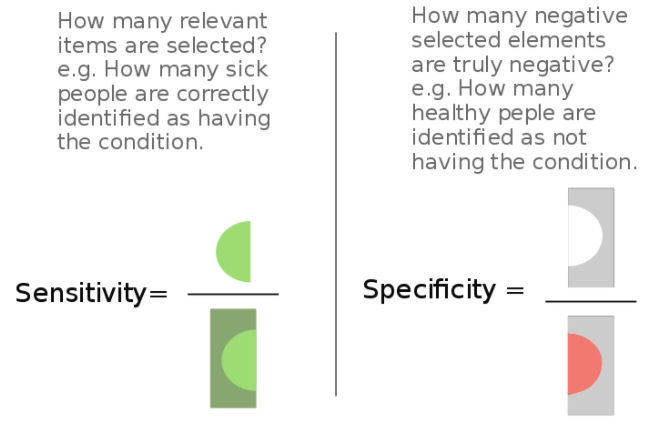
Sensitivity/True Positive Rate/Recall (R)

Fraction of positives predicted correctly (i.e., what percentage of all positive cases did your model capture accurately?). \(\frac{TP}{TP+FN}\)

/images/ml/ml_sensitivity_specificity.png
Specificity/True Negative Rate

Number of items correctly identified as negative as a percentage of total true negatives. This is the opposite of Recall. \(\frac{TN}{TN+FP}\)

Type 1 Error/False Positive Rate

Number of items wrongly identified as positive out of total true negatives. \(\frac{FP}{FP+TN}\)

Type II Error/False Negative Rate

Number of items wrongly identified as negative out of total true positives \(\frac{FN}{FN+TP}\)

F1 Score

This is the Harmonic Mean of Precision and Recall. It is a single score that represents both Precision and Recall. \(\frac{2 \times \text{P} \times \text{R}}{\text{P}+\text{R}}\)

Tip

  • Only use Accuracy when target variable classes are balanced (i.e., 80-20). Never use accuracy for imbalanced datasets.

  • Use Precision when it is absolutely necessary that all predicted cases are correct. For example, if it situation is to predict whether a patient needs open-heart surgery, you want to make sure you are correct as being wrong has a high cost (for the patient anyway)

  • Use Recall when it necessary to capture all possibilities that a case is True. For example, if you are identifying patients for quarantine for a highly contagious disease at an airport for an additional 10 minute screening, you would use Recall as the cost of letting the sick patient through is high.

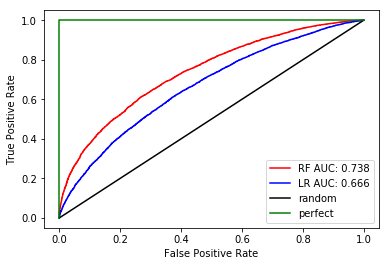
ROC-AUC

Receiver Operating Characteristic - Area under Curve

/images/ml/ml_auc_roc.png

Log-Loss

Log-loss involves the idea of probabilistic confidence for a specific class.

\begin{equation*} \text{LogLoss} =\frac{1}{N} \sum^{N}_{i=1} \sum^{M}_{j=1} y_{ij} \log (p_{ij}) \end{equation*}

\(y_{ij}\), indicates whether sample \(i\) belongs to class \(j\). \(p_{ij}\), indicates the probability of sample \(i\) belonging to class \(j\). Log Loss has no upper bound and it exists on the range \([0, \infty)\). Log Loss nearer to 0 indicates higher accuracy, whereas if the Log Loss is away from 0 then it indicates lower accuracy.

In general, minimising Log Loss gives greater accuracy for the classifier.

Cohen's Kappa metric

Metric that is useful for imbalanced classification

Bagging vs Boosting

Bagging and boosting are ensemble techniques that reduce errors and increase stability of the final model by combining multiple models. The principle idea is to group weak learners to form one strong learner. Errors from machine learning models are usually due to variance, noise or bias and ensemble techniques work to reduce variance and bias.

2 minute read…

Capital charge modelling for securitized products (SFA)

Capital modelling is a very important aspect of the financial industry that quants get involved in. After all, the role of a bank is as a financial intermediary to receive deposits and issue loans, and we've all heard of the bank runs during the Great Depression of the 1930s where by bank customers panic and start retrieving all their deposits from a bank. Such actions can cause a financial crisis, especially if it happens across multiple banks simultaneously.

10 minute read…

Fitting a volatility model on indices

Today a quant posed me a question:

If I had a sorted timeseries, how would I know if it was ordered correctly? What if it's in reverse?

After having an interesting conversation about how I would problem-solve the issue, he infomed me that a straightforward way was to fit a GARCH model, and that the model fit would be much higher if the timeseries was sorted in the right direction. While I wasn't quite sure of the econometric underpinnings of the solution, its not difficult to explore the idea.

In a previous post, we tried using the Google stock, and in this post we will try using an index, as per his suggestion. In this post, I've downloaded the following data from Ken French's data library

55 minute read…