Capital charge modelling for securitized products (SFA)

Capital modelling is a very important aspect of the financial industry that quants get involved in. After all, the role of a bank is as a financial intermediary to receive deposits and issue loans, and we've all heard of the bank runs during the Great Depression of the 1930s where by bank customers panic and start retrieving all their deposits from a bank. Such actions can cause a financial crisis, especially if it happens across multiple banks simultaneously.

Thus, its important that each bank ensures that they hold an optimal amount of capital in reserve. Having too little capital in reserve means that if an economic recession occurs, and customers start defaulting (i.e., not paying back) their loans, bank depositors can panic and trigger a bank run. Having too much capital in reserve means that the bank's balance sheet is not efficient and the banks equity shareholders might not be getting a sufficient return on equity (ROE).

Fortunately, we have statistical approaches to help us calculate the optimal amount of capital a bank needs to hold which is also regulated by reserve banks of most countries and the Basel Accords. This is called the Risk-Weighted Asset (RWA) calculation. RWA estimates are based on the Internal Ratings Based (IRB) approach based on the asymptotic single risk factor (ASRF) framework. The RWA is given as follows:

$$ \text{RWA} = 12.5 \times K \times EAD $$

RWA estimations for securitised assets¶

For securitized assets, the RWA is adjusted for the unique characteristics of securitized products as there are different tranches.

$$\text{RWA} = 12.5 \times CR \times EAD$$

$CR$ is the credit ratio, and $EAD$ is the exposure at default. $CR \times EAD$ gives us the total dollar risk-based capital requirement. Thus, the RWA is equal to the total dollar risk-based capital requirement multiplied by 12.5.

The two approaches are called:

• Simplified Supervisory Formula Approach (SSFA)
• Supervisory Formula Approach (SFA)

The SSFA is a simplified approach that results in a capital reserve estimate that is generally more conservative than the SFA. Thus, financial institutions will opt for the SFA approach when possible.

RWA estimations for securitized assets using the SFA approach¶

We discuss the RWA calculation for securitized assets here using the SFA approach as it is one of the most complicated capital modelling approaches on Wall St. It is more complicated than the SFA approach as it requires the statistical estimation of the probability of default (i.e., PD) and loss given default (i.e., LGD) of different replines/cohorts of the securitized product.

Some useful references that this write-up is based on is as follows:

• BCBS
• FED BCC13-7
• FED BCC13-5
• FED BCC14-3
• Moodys Analytics

The RWA calculation for securitized assets requires 7 inputs:

1. Capital charge ($K_{irb}$)
2. Underlying exposures (UE)
3. Tranche Percentage (TP)
4. Credit enhancement level (L)
5. Tranche thickness (T)
6. Effective number of exposures (N)
7. Exposure-weighted average loss-given-default (EWALGD)

The Capital charge ($K_{irb}$) is the most complicated parameter to estimate, and items 2 to 7 are usually based off the balance sheet characteristics of the securitization product and is obtained by the securitized product prospectus. Thus, minimal calculation or estimation is required for items 2 to 7.

Capital charge ($K_{irb}$)¶

The most important input that is often estimated statistically is $K_{irb}$, that is the capital charge for the underlying exposures plus the expected credit loss (ECL) as follows:

$$ K_{IRB} = K(PD_{i},LGD_{i})+PD_{i} \times LGD_{i} $$

• Capital charge for underlying exposures: $K(PD_{i},LGD_{i})$
• Expected Credit Loss (ECL): $PD_{i} \times LGD_{i}$

$K$ is the capital charge for underlying exposures. It is based upon the expected loss over a 1 year horizon conditional on a systematic risk factor with a value at the 99.9\% quantile of its probability distribution (i.e., systemic risk factor during a tail loss scenario).

$$ K(PD,LGD) = \left[LGD \times N \left( \frac{N^{-1}(PD)+\sqrt{R} \times N^{-1}(0.999)}{\sqrt{1-R}}\right)-( LGD \times PD) \right] $$

• $N(x)$ is the normal cumulative distribution, and $N^{-1}(x)$ is the inverse normal cumulative distribution.
• $R$ is the correlation parameter.
  • $R = 0.15$ for residential mortages
  • $R = 0.04$ for qualifying revolving exposures such as credit cards.
  • $R = 0.03+0.13 \times e^{-35\times PD}$ for other retail exposures

PD and LGD estimation¶

$K$ is calculated based on through-the-cycle probability of default ($PD_{TTC}$), and the maximum loss of the (i) through-the-cycle loss-given default ($LGD_{TTC}$) (ii) downturn loss-given-defult ($LGD_{DT}$).

$$ PD_{i} = \widetilde{PD_{TTC}} $$$$ LGD_{i} = \max (\widetilde{LGD_{TTC}},\widetilde{LGD_{DT}}) $$

PD and LGD estimates are estimated over large datasets where available (i.e., statistical, machine, deep learning techniques). These datasets can be loan-level, cohort-level, or balance-level data.

To comply with FED and BCC requirements, the minimum size of the dataset is follows:

Parameter	Wholesale (Years)	Retail (Years)
PD	5	5
LGD	7	5
EAD	7	5

Guidance from regulators is that the dataset must include a range of downturn and benign economic conditions, and selected downturn periods should not exceed 2 years.

For details on how PD and LGD is modelled, a related post is capital modelling as applied to securitized financial products

Data sources for PD and LGD¶

The following are common data sources used for calculationg PD and LGD:

• Loan/lease level data
• Static pool cohort
• Aging data
• Mapping approach (default rate)
• Mapping approach (loss rate)

Optimal $K_{IRB}$ estimate¶

The entire loan portfolio consists of different cohorts (i.e., replines) that are different portions of the portfolio of different balances and loan characteristics (i.e., PD, LGD). Any estimate of $K_{IRB}$ for the portfolio must be balance-weighted in order to take into account the balances and characteristics of each cohort sepearately.

$$ \bar{x} = \frac{\sum^{n}_{i=1} x_{i} \times BAL_{i}}{\sum^{n}_{i=1} BAL_{i}} $$

There are two ways to estimate $K_{IRB}$ for an entire loan portfolio. We either use a balance-weighted average of $K_{IRB}$, or a balance-weighted average of the PD and LGD inputs that are in $K_{IRB}$ formula.

Balance-weighted average $K_{IRB}$¶

Calculate a separate $K_{IRB}$ for each cohort $i$ to obtain $K_{IRB,i}$ so we use a balance-weighted average to obtain $K_{IRB}$ as follows:

$$ K_{IRB,1} = \overline{ K_{IRB} } $$

Balance-weighted average $PD_{i}$ and $LGD_{i}$ to obtain $K_{IRB}$¶

Calculate the balance-weighted $PD_{i}$ and $LGD_{i}$ to obtain $\overline{PD}$ and $\overline{LGD}$ to be used as inputs into the K_{IRB} formula as follows

$$ K_{IRB,2} = K(\overline{PD},\overline{LGD})+\overline{PD} \times \overline{LGD} $$

Using the balance-weighted average $K_{IRB,1}$ approach is the less conservative approach compared to $K_{IRB,2}$.

$$ K_{IRB,1} < K_{IRB,2} $$$$ \overline{ K_{IRB} } < K(\overline{PD},\overline{LGD})+\overline{PD} \times \overline{LGD} $$

This is because the $K$ formula is a concave function and Jensen's Inequality. The figure below depicts this clearly.

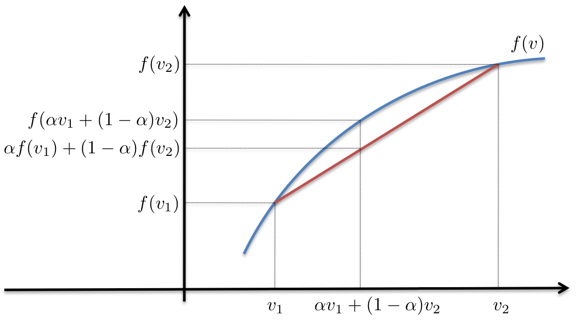
As can be seen from the above graphic, the balance-weighted inputs into the formula $f$ will always be greater than the balance-weighted of the function applied to the inputs as shown below

$$ \alpha f(v_{1}) + (1-\alpha) f(v_{2}) < f[ v_{1} + (1-\alpha) v_{2}] $$

However, capital quants be pressured by the business to produce lower capital numbers and will therefore take advantage of Jensen's inequality to produce less consservative capital reserve estimates.

What's the magnitude of the impact between both approaches on the $K_{IRB}$ output?¶

The lower the capital reserve estimates, the greater the amount of capital that can be deployed to the financial institutions loans business. However, what is the magnitude of the impact to the bottom-line capital requirement number between using balance weighted average $K_{IRB}$ vs balance weighted average $PD$ and $LGD$ as inputs into $K_{IRB}$? From, it depends on the curvature of the $K_{IRB}$ line, and the distance between $v_1$ and $v_2$. Thus, if the securitized portfolio of credit products exhibits a large variance in $PD$ across different replines/cohorts, the difference between the curved and straight line will be greater.

Thus, if you are evaluating the $K_{IRB}$ model output, it is important to validate the magnitude of the difference between both approaches.

$K_{irb}$ calculation¶

Importing all required Python modules

The $K_{IRB}$ calculation that can be found from Advanced IRB. We can see that correlations have the largest impact on $K_{IRB}$. For example, lower correlations mean lower $K_{IRB}$. Some might look at $K_{IRB}$ and wonder why it is a concave curve going downwards meaning that at higher $PD$, the $K_{IRB}$. It is important to understand that $PD$ is not meant to be too high (i.e., greater than 20%), so we use $K_{IRB}$ up to the maximum point of the quadratic curve.

Producing plot of $K_{IRB}$¶

Correlation parameter for large enterprises

Correlation parameter for Small-to-Medium enterprises

RWA estimations for securitized assets using the SSFA approach¶

The SFA is a more straight forward calculation that the FED provides an example spreadsheet in FED SR15-4. The inputs to the calculation are balance sheet information based on the characteristics of the securitizated product.

The Simplified Supervisory Formula Approach (SSFA) is used when the financial institution has insufficient data to apply the SFA approach. The SSFA is generally more conservative than the SFA approach.

@param kG: weighted average total capital requirement of underlying exposures
@param w: ratio of sum of defaulted amounts to underlying exposure
@param a: attachment point of exposure. Threshold where credit losses start to be allocated to the bank's exposure.
The ratio of underlying exposures that are subordinated to the exposure of the bank, to the current dollar amount of underlying exposures (decimal value between 0 to 1)
@param d: detachment point of exposure. Threshold where credit losses will result in total loss of bank's exposure. parameter A+ artio of (decimal value between 0 to 1)
@param p: supervisory calibration parameter. 0.5 (1.5) for securitization (resecuritization) exposures
@return